Oligarchy and Democracy

The desire for power may either be a universal human drive, an evolutionary outcome or to autonomously control one’s outcome and self-actualize as described by Nietzsche. Whatever the reason may be, the desire for power has shaped the history of humankind – social hierarchies, political systems and economic relations. But power is not distributed uniformly among the members of society. From tribal societies to modern state, power is often concentrated on the select few who dominate the many. There is the continuous struggle between the elites and commons that can be seen as a conflict between those seeking to protect existing power and those striving to gain power or challenge it.

Aristotle argued that the most virtuous form of governance is when select few individuals - noble by birth and distinguished by intellectual and moral character govern over the populace. Unfortunately, these elites often succumb to fulfillment of their private interests over the common good and this ideal form of governance deteriorates to oligarchy. Aristotle defined Oligarchy as, “Wherever men rule by reason of their wealth, whether they are few or many, that is an oligarchy.” This definition differentiates the rich from oligarchs i.e. Not all richs are oligarchs. He viewed oligarchy as a deviant form of rule by the elites that occur when elites become corrupt. In modern times, Robert Michels has made influential contribution to understanding oligarchy. His “Iron law of Oligarchy” states that “Who says Organization, says oligarchy” explains that organizations regardless of how democratic they are initially, inevitably develop into oligarchic. This article discusses (i) oligarchy as a default setting of society (ii) the modern oligarchs - financial and techno-oligarchs (iii) democratic backsliding – an output of oligarchy?

Oligarchy, inevitable feature of society?

Is society oligarchic by nature? To answer this question, we must go back to the earliest days of human history. Anthropologists argue that earliest human societies were relatively egalitarian in terms of status and resources. Rueden (2020) , Boehm (1999) , Erdal & Whiten (1996) claimed that hunter gatherer societies were egalitarian in nature. Boehm (1999) in his seminal work “Hierarchy in the Forest: The evolution of egalitarian behaviour” explained the “reverse dominance hierarchies” nature of early human societies. The band members would form coalition that suppressed anyone trying to become dominant. They would hold-down their would be alphas through disobediance, ostracism or execution (Boehm, 1993) .

However, the shifts in ecological and demographic conditions especially agriculture weakened the constraints on coercion (Rueden, 2020) . Social dynamics changed with the ability to accumulate productive land, grains and domesticated animals. Earle (1997) , Flannery & Marcus (2012) argued that surplus storage and strategic control of specific resources (land) created chiefly authority in early Polynesian, Andean and European Societies. The Chiefs used the strategic control over resources not for communal benefit but to create debt and obligation. The competition to control over the fertile land increased due to the population pressure which resulted into warfare and ultimately the formation of centralized polity. Centralized polity formed faster in areas with circumscribed agricultural land (Carneiro, 1970) . The new political economies mobilized the surplus to support administrators, soldiers and dependent artisans. The mobilization of surplus could either result in further increase in mobilization of surplus to support the more administrators and soldiers thereby creating a self-reinforcing system or systemic collapse (Wright, 2006) . The ruling class could strengthen their position in case of self reinforcing system. The existence of ruling class doesn’t necessarily imply an oligarchic structure. However, historical evidence suggests that in many ancient civilizations, economic and political powers were usually concentrated on the hands of wealthy elites. In Sumer, power was shared between temple and merchant families while between palace and warrior aristrocrats in Mycenaean Green. Powerful wealthy families often maintained control behind the facade of monarchy. History reveals that there is often power concentration on the hands of few. But what does scholars say about elite dominance?

Gaetano Mosca, Italian Political Scientist in his Theory of Ruling Class (1986) argued that small, organized minority ruling class governs over the larger, disorganized majority (the ruled). He argued that even in democracy, power is often exercised by small group of elites. The ruling class justifies its power to the masses by legitimizing their ideology. Vilfredo Pareto’s Circulation of Elites explained that “history is graveyard of aristocracies”. The circulation of elites occur in any society either democratic or autocratic. He argued that political change occurred when one elite is replaced by other rather than through masses overthrowing the elites. Though Mosca and Pareto have not exclusively defined these elites as oligarchic but they have argued that small group of elites dominate over the masses. Robert Michels in his book Political Parties: A Sociological Study of Oligarchical tendencies of Modern Democracy (1911) propose the “Iron law of Oligarchy.” He argued that every organization, whether democratic or not, inevitably evolves into an oligarchy. Michels as a member of Social Democratic Party, observed firsthand that how this democratic party had become rigid and bureaucratic over a period of time governed by small group of elites. He explained that this oligarchic tendency is due to (i) adminitrative factors – division of labor, centralized command, technical expertise (ii) incompetence of masses – most of the members are poorly informed and lack ability to understand, (iii) psychological factors – leaders develop taste for power and position while masses feel grateful to their leaders reinforcing leader’s power and legitimacy (cult of veneration among masses).

Contrary to Michels arugment that oligarchy is unavoidable, advocates of Pluralism – Robert A. Dahl, David Truman, Seymour Martin Lipset argue that power is polycentric. They didn’t claim that democracy is free of elites but institutional structure and group competition can hinder the oligarchic dominance. David Truman in his book The Governmental Process (1951) wrote the formation of counter-organization may not occur immediately but it is inevitable. Competing interest groups continuously interact eachother to counterbalance one another to reach an equilibrium. Like Truman, Robert Dahl in Who Governs? Democracy and Power in an American City (1961) argued that power¹ is distributed among the competing groups – unions, civil society, media, business organizations. He used the term “polyarchy” indicating multiple power centers. The distribution of power among competing groups ensures that there is no monopoly of power by an elite group. Citizens can exercise their power not only through ballot box but also through group membership and advocacy. The problem with this pluralist ideas is that unlike elites, oligarchs can have varying political agenda but they all agree on wealth and property defense like lowering taxes as per Jefferey Winters.

The question “Is society oligarchic by nature?” is still unanswered. We have two opposing theories – classical elite theorists support elite dominance in society while pluralists support the idea of polycentric society. May be the question can’t be simply answered with yes or no. Humans have innate desire for wealth and power which might be a reason for the societal drift towards oligarchy. Historically, most of the societies were governed by elites. Organizational necessities, the political utility of accumulated wealth, structural inertia, elite social networks can strengthen elite dominance in societies. However, democratic mechanisms – strong and active civil society, independent media, rule of law can mitigate these oligarchic tendencies. Diefenbach (2018) argues that the “iron law of oligarchy” is neither iron nor law — that democratic organisations can indeed maintain internal democracy and avoid oligarchic drift by design. What we can conclude is that society possess oligarchic tendencies, but it is not oligarchic by nature. It is contingent on the balance between elite dominance and democratic system. Oligarchy rises as democracy weakens.

The Modern Oligarchs – Techno and Financial Oligarchs

Oligarchs in ancient societies emerged as a consequence of social hierarchy. Individuals considered “nobles” were endowed with hereditary privilege, royal patronage – with large area of fertile land. In Ancient Greece, Eupatridae – the noble born, had large area of land and tangible assets. The wealth would help them to fund liturgy, trierarchy and maintain network of clientelism. The nobles would secure administrative or advisory positions within the royal court which would further enable them to create more wealth. Those elites who controlled large estate would also dominate councils like Areopagus (Morris & Powell, 2004) .

Unlike the oligarchy in ancient societies whose authority was derived from birth, kinship and hereditary privilege, the modern oligarch’s power came from wealth accumulation, networks and political patronage. However, this shift from hereditary to achieved status is not absolute. Inherited privilege is still prevalent in political (Marcos family in Philippines, Sheikh-Wazed family in Bangladesh) and economic (Lee family in South Korea, Rockefeller family in USA) dynasties. To account for the features of these modern oligarchs, David Lingelbach and Valentina Rodriguez Guerra reworked Aristotle’s definition and defined oligarch as “someone who secures and reproduces wealth or power, then transforms one into the other.” This definition highlights the elite capacity to convert power into wealth and vice versa. Russia’s Sale of the Century is the example of how elites with political patronage got control of major state-owned enterprises. During mid-1990s, loan-for-shares scheme was introduced. The government pledged shares of valuable state-owned enterprises – primarily in oil, metals and telecommunication sectors as collateral. The government defaulted on the loans and the pledged shares were auctioned by the banks. However, politically connected elites obtained the ownership of these enterprises at discounted prices through insider-controlled auctions. Vladmir Potanin secured Norilsk Nickel, Mikhail Khodorkovsky – Yukos Oil Company, Boris Berezovsky – Sibneft, Mikhail Fridman – Tyumen Oil Company.

Simon Johnson argues that modern oligarchs have arisen especially in financial and technological sector in recent decades. First form of oligarchy have emerged in financial sector, especially banks and investment firms that have become too big to fail. Large banks and investment firms take more risks because they operate under implicit guarantee that government bail them out as evidenced during 2007-08 Financial crisis. The shift towards “financialized capitalism” has increased the influence of financial elites over policymaking (Epstein, 2005) . Second oligarch is techno-oligarchs who control digital infrastructure and data. Leaders of tech corporations like Apple, Microsoft, Nvidia, Facebook are powerful enough to influence consumers’ behaviour and politico-economic decisions. People are offered “free services” to get hooked to the social media platform but the hindsight, they collect every user’s data. They possess capacity to influence users’ beliefs on certain topics by prioritizing or suppressing particular content in user’s feed. The Cambridge Analytica – political consulting firm collected personal data from Facebook users and used the information to influence the outcome of 2016 US presidential election. Techno-oligarchs have power to challenge traditional governance and influence the political and economic systems through their control of data, communications and technological infrastructures. The emergence of artificial intelligence has further strengthened concentration of power, enabling firms to dictate technological trajectories while advocating for minimal regulatory oversight (Acemoglu & Johnson, 2023) .

Democratic Backsliding – an output of oligarchy?

V-Dem Institute’s Democracy Report 2025 showed that there is significant rise in democratic backsliding² worldwide. For the first time in two decades, the world has fewer democracies than autocracies, i.e. 91 autocracies and 88 democracies in 2024. Moreover, the share of world’s population living under liberal democracy is the lowest in 50 years, now comprising less than 12% of world population. But what causes democratic backsliding? Freedom House states that democracy is under attack by populist leaders and groups that reject pluralism and demand unchecked power to advance the particular interests of their supporters, usually at the expense of minorities and other perceived foes. In this section, this article discusses two questions – (i) Is oligarchy a cause of democratic backsliding? (ii) If yes, how does it do so?

Does oligarchy cause democratic backsliding? Empirical evidence shows that when power – economic and political is concentrated on the hands of few, democratic institutions and mechanisms tend to erode. Oligarchic power is rooted in the wealth, and these oligarchs are united by “wealth defense” according to Jeffrey Winters. Unlike in democracy that tries to achieve a more egalitarian distribution of resources, oligarchy attempts to create a non-level playing field and monopoly position for politically powerful elites through entry barriers (Acemoglu, 2008) . Wealthy elites lobby for policies like lower taxation and often succeed. Monopoly position coupled with tax breaks increases the wealth of the elites which further intensifies the inequality. Top 1% own 47.5% of all the world’s wealth in 2023 according to Global Wealth Report 2024. Extreme inequality disincentivizes elites to support democratic system because of perceived threat of redistribution (Acemoglu & Robinson, 2006) . Rau & Stokes (2025) argued that income inequality is strong and highly robust predictor of democratic erosion. They concluded that probability of democratic erosion rise from single digits in the most equal countries to more than 30% in the most unequal ones. The goal of oligarchs may not be to weaken democracy but their actions for wealth defense and accumulation ultimately weaken the democratic institutions, systems and processes.

Income Inequality & Probability of Democratic Erosion

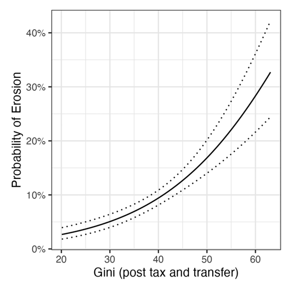
Source: Rau and Stokes (2025)

How do oligarchs weaken democracy? First, oligarchs weaken democracy by influencing policy outcomes through lobbying and political donations. Oxfam (2024) found that collective spending of 182 largest companies on lobbying was 746 million dollars in 2022 i.e. an average of 4.5 million dollars per company. Another study conducted by Oxfam (2016) found that for every 1 dollar spend on lobbying by the largest 50 US public companies, they received 130 dollars in tax breaks and more than 4000 dollars in federal loans, loan guarantees, and bailouts. Boas et. al., (2011) found that firms would be awarded projects at least 8.5 times their contributions provided that the federal deputy candidate they supported from the ruling workers’s party win the election in Brazil. Lobbying can generate financial returns far greater than the amount spent which assist elites to increase their wealth. The economic power translates to political power resulting into the political inequality which is contratry to the equality principle of democracy. Gilens & Page (2014) found that economic elites and organized groups have strong influence on US government policy while average citizens have little or no influence. Elsasser et. al., (2021) found similar conclusions in Germany.

Second, oligarchs often control the media to influence the public discourse to achieve their interests – political and business. The ability of media – TV stations, newspaper to deliver true and unbiased information erodes when it is influenced or controlled by oligarchs. In Italy, Silvio Berlusconi – former prime minister and a media tycoon, used his ownership of MediaSet, a media holding company to gain political power. Media is often used by oligarchs as a tool to shape public perspective, create a positive image of themselves and even distract public from their wrongdoings. The growth of media controlled or linked to oligarchs is growing throughout the world. A three year study performed by Organized Crime and Corruption Project in Eastern Europe, the Balkans and the former Soviet Union found that majority of media are linked to politically connected businessman, persons with criminal records and shell companies. Beyond the traditional media, modern techno-oligarchs have the control of social media which enable them to act as the modern gatekeepers of information. Platforms like Facebook, Tiktok, X (formerly Twitter), Youtube can influence public discourse – amplyfying certain voices while marginalizing others. Cambridge Analytica Scandal proved the strength of social media to manipulate voter behaviour.

Third, oligarchs weaken the checks and balance mechanisms of democracy through state capture. Hellman, Jones, & Kaufmann (2000) explained that wealthy and politically linked elites shape the rules of the game – manipulate laws and regulations, and influence state institutions to their own advantage, at considerable social cost, creating a “capture economy”. State capture can occur through legislation of favourable laws and regulations, and influence in the judicial, regulatory and administrative body for private gains. The case of Gupta family in South Africa is the most documented example of modern state capture. The Zondo Commission explained that the Gupta family in collusion with the then-president Jacob Zuma was able to capture state through (i) appointment of collaborators in senior key positions, (ii) weaken the law enforcing agencies, (iii) weaken the parliamentary oversight, and (iv) influence and control the media.

Fourth, oligarchs influence electoral competitiveness through donations. The integrity of election system is a key to healthy, strong and resilient democratic system. The election competitiveness has eroded due to the concentrated wealth, systematically undermining the level playing field required for democratic elections. The outcome of the election has been found to depend on the candidates’ ability to spend on election campaign. In 2020, 89.1% of House candidates and 69.7% of Senate Candidates that outspent their opponents won their election as per Center for Responsive Politics. Similar conclusions have been found in Brazil (Samuels, 2001) , Ukraine (Matuszak, 2012) . This creates advantage for wealthy candidates or those supported by wealthy donors. Once elected, political donations often amplify the voices of wealthy donors, so that policies are aligned with the interests of donors.

Policies to check the power of Oligarchs

Oligarchy can be the result of a weakened democracy or the cause of the weakening democracy. From ancient chiefs to modern techno-financial oligarchs, wealth is the primary source of power. Income inequality reinforces the power concentration on the hands of oligarchs. Political inequality affects the policy outcome in favor of elites. Because the power of oligarchs is primarily derived from their wealth, economic policies that can tackle income inequality can be effective tools to control their power. First, progressive taxation can be effective tool to reduce inequality (Piketty, 2014) – particularly direct income taxes. The government revenue from the progressive taxation can be redirected towards social welfare system. Second, anti-monopoly and competition policies can prevent the emergence of large monopolies that have huge political power. Larger monopolies possess significant leverage to influence policy making through their capacity to threaten investment deferral or withdrawal as well as through the control of information flows, especially by tech corporations. Third, setting up transparency mechanisms in procurement contracts and political donations can reduce covert channels through which oligarchs exert political influence. Fourth, strengthening labor rights and ensuring formation of labor unions can lead to better wage bargaining, which serves as a tool to reduce wealth concentration.

The oligarchic tendencies in the society reinforced by the accumulation of wealth and power continuously challenge the democracy. Well designed economic policies together with strong democratic institutions can minimize the capacity of wealthy elites to dominate and influence the political processes. The resilience of democracy depends on the ability of the state and citizens to prevent the convergence of economic and political power on the hands of few.

Footnotes